Tutorial Cases
Case Description
This validation case simulates the inviscid transonic gas flow through a Convergent-Divergent (CD) nozzle (JPL nozzle).
The axisymmetric simulation aims to validate the solver's capability to simulate supersonic flows and capture shock waves in the flow field.
The nozzle geometry is taken from Back et. al, and the inlet and throat curvature points is generated in MATLAB. These data points
are then provided to modify the boundaries of domain block in the blockMeshDict. The MATLAB code is available with the case files.
The CD nozzle mesh along with the boundaries marked are shown in the figure and the boundary conditions are presented in the table.
Initially pressure and temperature is 1.0 bar and 300 K and is set to be uniform throughout the domain. The specific heat capacity
of the gas is 1.07 J/kg.K and the ideal gas equation of state is employed. The molecular weight of the gas is 28.786 kg/kmol.
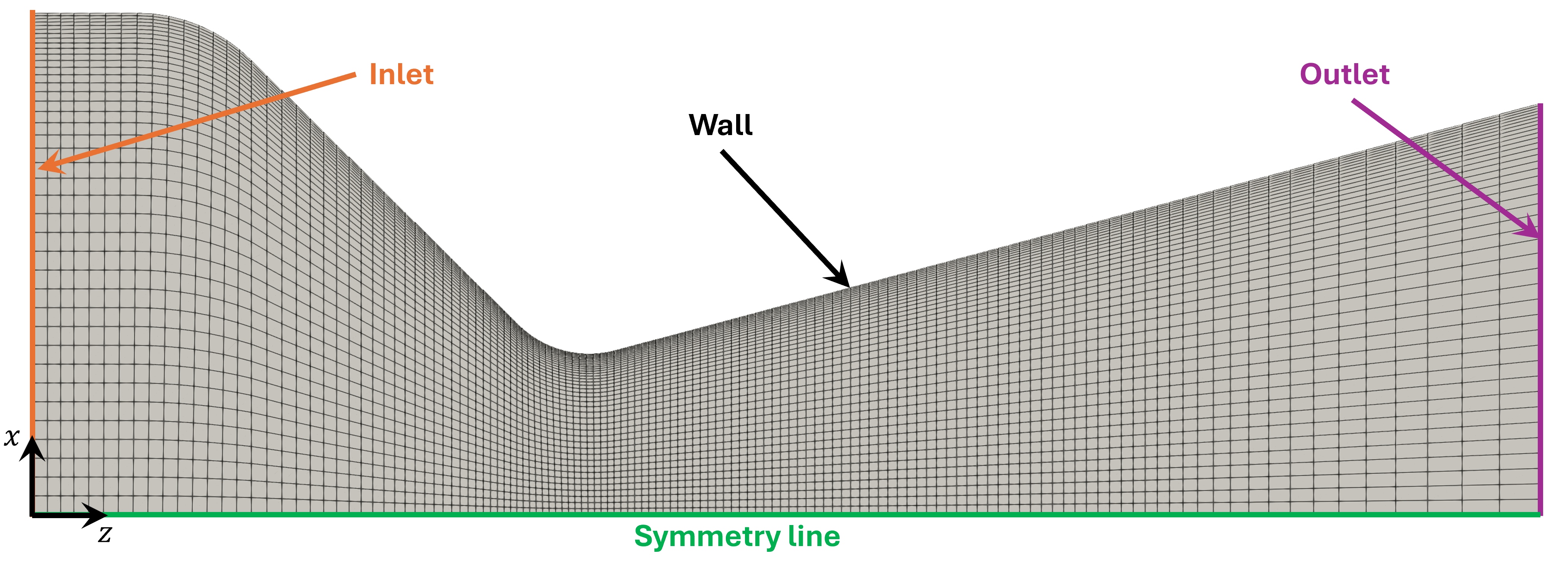
JPL Nozzle Mesh with Boundaries
Boundary Conditions
| Variables | Inlet | Outlet | Wall | Wedge faces |
|---|---|---|---|---|
| $P$ | Total Pressure (10.34 bar) | zeroGradient | zeroGradient | cyclic |
| $\boldsymbol{u}_g$ | PressureDirectedInletVelocity (inlet direction: +z axis) | zeroGradient | Slip | cyclic |
| $T_g$ | Total Temperature (555 K) | zeroGradient | zeroGradient | cyclic |
Numerical Schemes
Initially, the simulation is conducted till steady state (t = 0.01 s) with first orderupwind scheme for all
the convective terms. To improve the accuracy the the convective schemes are updated to vanLeer scheme for
all the convective terms. The generalized Crank Nicolson scheme is used for time integration for second order
accuracy and stability.
Instructions to Run the Simulation
Before beginning, ensure you source the native OpenFOAM-v2112 bashrc file and the RocPerf bashrc file.
The case file is available in the directory tutorials/JPL-Nozzle. Copy the case file to your working directory. To mesh the geometry, run:
blockMesh
You can run the simulation in either serial or parallel mode:
Option A: Serial Run
rocketMotor
Option B: Parallel Run
First, perform mesh decomposition, then run with MPI (default is 8 processors):
decomposePar
mpirun -np 8 rocketMotor -parallel
Note: The number of processors can be adjusted in the decomposeParDict file.
To obtain accurate simulation results (as shown in the plots below), simply double the mesh size in the
blockMeshDict file before running the mesh generation.
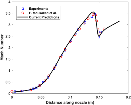
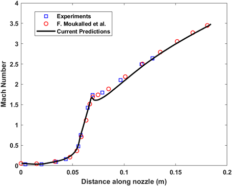
Results
The predicted centreline Mach number and the wall Mach number is plotted with experimental data and the computational data from F. Moukalled et al.
 |
 |
References
- Moukalled, F., Darwish, M., and Sekar, B., “A Pressure-Based Algorithm for Multi-Phase Flow at All Speeds,” Journal of Computational Physics, Vol. 190, No. 2, 2003, pp. 550–571. doi: 10.1016/S0021-9991(03)00297-3.
- Back, L., and Cuffel, R., “Detection of Oblique Shocks in a Conical Nozzle with a Circular-Arc Throat,” AIAA Journal, Vol. 4, No. 12, 1966, pp. 2219–2221. doi: 10.2514/3.3881.
- Chang, H. T., Hourng, L. W., Chien, L. C., and Chien, L. C., “Application of Flux-Vector-Splitting Scheme to a Dilute Gas-Particle JPL Nozzle Flow,” International Journal for Numerical Methods in Fluids, Vol. 22, No. 10, 1996, pp. 921–935. doi: 10.1002/(SICI)1097-0363(19960530)22.
Case Description
This validation case simulates the inviscid transonic dusty gas flow in a Convergent-Divergent (CD) nozzle (JPL nozzle). The axisymmetric simulation aims to validate the solver's capability to model gas-particle interactions. The nozzle geometry and mesh is same as the previous case. The particle phase is introduced at the inlet. The boundary conditions for the gas and particle phase flow variables are presented in the table. Initial condition is taken to be steady state solution of gas phase from the previous tutorial. The particle phase volume fraction is initially zero. The gas phase properties remains same as the previous case. The particle phase density is 4004.62 kg/m^3 and the specific heat capacity of the particle phase is 1.38 kJ/kg.K . The diameter of the particle is 20 $\mu$m. The velocity and temperature slip at the inlet is assumed to be zero in this case. The coefficient of drag and Nusselt number correlation used for this validation simulation are given by, $$ C_D = \frac{24}{Re_p}\left(1 + 0.15Re_p^{0.687} + \frac{0.0175Re_p}{1 + 4.25\times 10^4Re_p^{-1.16}}\right) $$ $$ Nu = 2 + 0.459Re_p^{0.55}Pr^{0.33} $$
JPL Nozzle Mesh with Boundaries
Boundary Conditions
| Variables | Inlet | Outlet | Wall | Wedge faces |
|---|---|---|---|---|
| $P$ | Total Pressure (10.34 bar) | zeroGradient | zeroGradient | cyclic |
| $\boldsymbol{u}_g$ | PressureDirectedInletVelocity (inlet direction: +z axis) | zeroGradient | Slip | cyclic |
| $\boldsymbol{u}_p$ | sameAs - gas phase ($\boldsymbol{u}_g = \boldsymbol{u}_p$) | outletInlet (no reverse flow) | Slip | cyclic |
| $T_g$ | Total Temperature (555 K) | zeroGradient | zeroGradient | cyclic |
| $T_p$ | sameAs - gas phase ($T_p = T_g$) | zeroGradient | zeroGradient | cyclic |
| $\alpha_g$ | zeroGradient | zeroGradient | zeroGradient | cyclic |
| $\alpha_p$ | massLoadingFraction ($X_p = 0.3$) | zeroGradient | zeroGradient | cyclic |
Numerical Schemes
The convective terms are discretized using second order shock capturingvanLeer scheme. The generalized Crank Nicolson scheme is used for time integration for second order
accuracy and stability.
Instructions to Run the Simulation
Before beginning, ensure you source the native OpenFOAM-v2112 bashrc file and the RocPerf bashrc file.
The case file is available in the directory tutorials/JPL-TwoPhase-Nozzle. Copy the case file to your working directory. To mesh the geometry, run:
blockMesh
You can run the simulation in either serial or parallel mode:
Option A: Serial Run
rocketMotor
Option B: Parallel Run
First, perform mesh decomposition, then run with MPI (default is 8 processors):
decomposePar
mpirun -np 8 rocketMotor -parallel
Note: The number of processors can be adjusted in the decomposeParDict file.
The specific impulse and characteristic velocity can be computed from the thrust and mass flow rate at the outlet patch. To obtain mass flow rate of gas and particle phase and the thrust for each time step, run:
postProcessRocket
This will generate a csv file containing mass flow rates and thrust for each time step, which can be further used to calculate specific impulse and $C^*$ as, $$ C^* = \frac{P_cA_t}{\dot{m}_{gas} + \dot{m}_{particles}} \hspace{20pt} I_{\text{sp}} = \frac{F}{(\dot{m}_{gas} + \dot{m}_{particles})g_0} $$
To obtain accurate simulation results (as shown in the plots below), simply double the mesh size in the
blockMeshDict file before running the mesh generation.
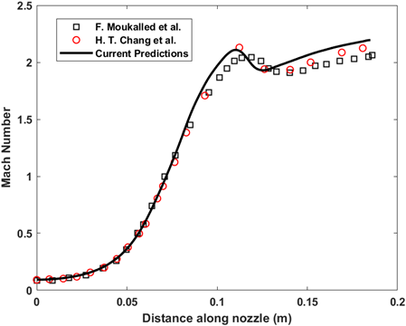
Results
The predicted centreline Mach number and the wall Mach number is plotted with experimental data and the computational
data from F. Moukalled et al. A similar analysis can be repeated for 2 $\mu$m particle size. The particle size
can be changed from the phaseProperties file in the constant folder.
 |
 |
The thrust and specific impulse of the JPL nozzle computed from the simulations are presented in this table.
| Simulation | Gas-phase Thrust $(\text{N})$ | Total Thrust $(\text{N})$ | Mass flow rate $(\text{kg/s})$ | $I_{\text{sp}} (\text{s})$ | |
|---|---|---|---|---|---|
| Computed | Chang et. al., 1996 | ||||
| Pure gas phase | 2097 | 2114 | 2097 | 2.191 | 97.6 |
| Gas-particle $(2.0 \mu\text{m})$ | 1630 | 1636 | 2198 | 2.635 | 85.35 |
| Gas-particle $(20.0 \mu\text{m})$ | 1870 | 1948 | 2230 | 2.956 | 76.9 |
References
- Moukalled, F., Darwish, M., and Sekar, B., “A Pressure-Based Algorithm for Multi-Phase Flow at All Speeds,” Journal of Computational Physics, Vol. 190, No. 2, 2003, pp. 550–571. doi: 10.1016/S0021-9991(03)00297-3.
- Back, L., and Cuffel, R., “Detection of Oblique Shocks in a Conical Nozzle with a Circular-Arc Throat,” AIAA Journal, Vol. 4, No. 12, 1966, pp. 2219–2221. doi: 10.2514/3.3881.
- Chang, H. T., Hourng, L. W., Chien, L. C., and Chien, L. C., “Application of Flux-Vector-Splitting Scheme to a Dilute Gas-Particle JPL Nozzle Flow,” International Journal for Numerical Methods in Fluids, Vol. 22, No. 10, 1996, pp. 921–935. doi: 10.1002/(SICI)1097-0363(19960530)22.
Case Description
This simulation case investigates the internal ballistics and multi-phase flow dynamics within a lab-scale rocket motor utilizing frozen nano-aluminum water (ALICE) propellant. Rather than modeling the transient process of propellant grain regression, this simulation focuses on a statistically steady-state 'snapshot' during the firing duration. By treating the grain geometry as fixed and the burning surface as a mass injection boundary, the simulation provides high-fidelity insights into the internal flow dynamics. The 2D axisymmetric mesh and the boundary conditions for the lab-scale rocket motor are shown in Figure 3.1.
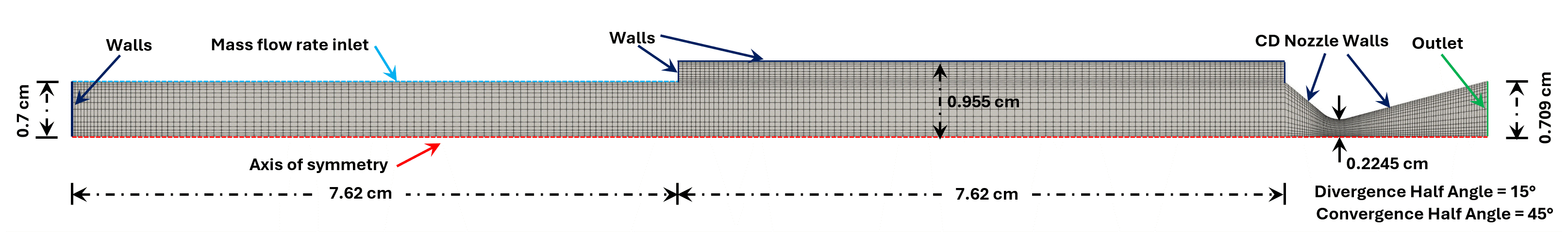
Fig 3.1: 2D Axisymmetric Mesh and Boundary Conditions of the Lab-Scale Rocket Motor.
For the steady-state simulation, the gas phase mass flow rate at the propellant grain interface is set to $0.1 \text{ g/s}$ with an associated particle mass fraction of $0.7194$. The adibatic flame temperature of the ALICE propellant, at an equivalence ratio of $0.943$ and a assumed combustion efficiency of $70 \%$,is $2270 \text{ K}$. The gas and particle phases are assumed to enter the simulation domain at the same velocity and at a temperature of $2270 \text{ K}$. The particle diameter is taken as $80 \text{ nm}$. For further details regarding the propellant, rocket motor firing experiments, and computational methodology, readers may refer to Risha et. al., (2014) and Venukumar et. al., (2025). For simplicity, thermophysical properties for both phases are assumed constant. The gas phase is defined by a specific heat of $10000 \text{ J/kg}\cdot\text{K}$, a molecular weight of $2.9 \text{ g/mol}$, a dynamic viscosity of $1e^{-4} \text{ Ns/m}^2$, and a Prandtl number of $0.7$. The particle phase density is $3950 \text{ kg/m}^3$ and the specific heat is $1800 \text{ kJ/kg}\cdot\text{K}$. Interphase momentum exchange is governed by the Loth drag model to account for compressibility and rarefaction effects, while gas-particle thermal exchange is modeled via the Ranz-Marshall correlation, modified by Kavanau’s correction factor to incorporate rarefaction effects.
Boundary Conditions
| Variables | Inlet/Propellant surface | Outlet | Wall | Wedge faces |
|---|---|---|---|---|
| $P$ | fixedFluxPressure | zeroGradient | fixedFluxPressure | cyclic |
| $\boldsymbol{u}_g$ | gasFlowRateInletVelocity ($0.1 \text{ g/s}$) | zeroGradient | noSlip | cyclic |
| $\boldsymbol{u}_p$ | sameAs - gas phase ($\boldsymbol{u}_g = \boldsymbol{u}_p$) | outletInlet (no reverse flow) | noSlip | cyclic |
| $T_g$ | $2270 \text{ K}$ | zeroGradient | zeroGradient | cyclic |
| $T_p$ | sameAs - gas phase ($T_p = T_g$) | zeroGradient | zeroGradient | cyclic |
| $\alpha_g$ | zeroGradient | zeroGradient | zeroGradient | cyclic |
| $\alpha_p$ | massLoadingFraction ($X_p = 0.7194$) | zeroGradient | zeroGradient | cyclic |
Numerical Schemes
The convective terms are discretized using second order NVD scheme -limitedLinear 1.0. The generalized Crank Nicolson scheme is used for time integration for second order
accuracy and stability.
Instructions to Run the Simulation
Before beginning, ensure you source the native OpenFOAM-v2112 bashrc file and the RocPerf bashrc file.
The case file is available in the directory tutorials/Steady-ALICE-motor. Copy the case file to your working directory. To mesh the geometry, run:
blockMesh
You can run the simulation in either serial or parallel mode:
Option A: Serial Run
rocketMotor
Option B: Parallel Run
First, perform mesh decomposition, then run with MPI (default is 8 processors):
decomposePar
mpirun -np 8 rocketMotor -parallel
Note: The number of processors can be adjusted in the decomposeParDict file.
The specific impulse and characteristic velocity can be computed from the thrust and mass flow rate at the outlet patch. To obtain mass flow rate of gas and particle phase and the thrust for each time step, run:
postProcessRocket
This will generate a csv file containing mass flow rates and thrust for each time step, which can be further used to calculate specific impulse and $C^*$ as, $$ C^* = \frac{P_cA_t}{\dot{m}_{gas} + \dot{m}_{particles}} \hspace{20pt} I_{\text{sp}} = \frac{F}{(\dot{m}_{gas} + \dot{m}_{particles})g_0} $$
To obtain higher resolution of flow dynamics, increase the mesh size in the
blockMeshDict file before running the mesh generation.
References
- Risha, G. A., Connell Jr, T. L., Yetter, R. A., Sundaram, D. S., and Yang, V., “Combustion of Frozen Nanoaluminum and Water Mixtures,” Journal of Propulsion and Power, Vol. 30, No. 1, 2014, pp. 133–142. doi: 10.2514/1.B34783.
- Venukumar, G., and Sundaram, D. S., “Computational Study of Propulsive Performance of Frozen Nano-Aluminum and Water (ALICE) Mixtures,” Journal of Propulsion and Power, Vol. 41, No. 3, 2025, pp. 330–346. doi: 10.2514/1.B39541.
Case Description
This simulation case investigates the internal ballistics and multi-phase flow dynamics within a lab-scale rocket motor utilizing frozen nano-aluminum water (ALICE) propellant. The motor and grain dimensions are derived from experimental data. A center-perforated propellant grain is considered, and the entire firing duration of the rocket motor—including propellant surface regression—is simulated. The 2D axisymmetric mesh and the boundary conditions for the lab-scale rocket motor are shown in Figure 4.1.
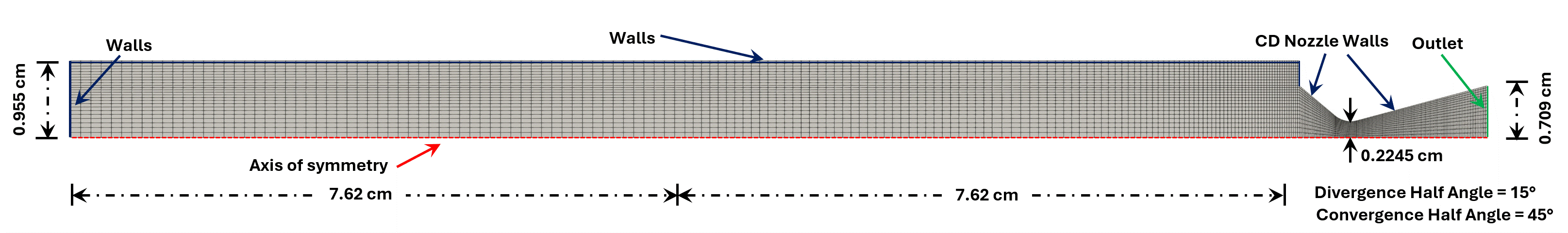
Fig 4.1: 2D Axisymmetric Mesh and Boundary Conditions of the Lab-Scale ALICE Rocket Motor.
The propellant surface regression is tracked using an interfaceTrackingModel of type,
entrainedInterfaceMotion. This requires the propellant burning rate to be expressed according
to St. Robert’s Law; the burning rate pre-exponential factor and pressure exponent serve as inputs for
this model. For the ALICE propellant with an equivalence ratio of $0.943$, the burning rate is
expressed as (Connell Jr et. al., 2012):
$$
r_b [\text{cm/s}] = 0.991\left(P[\text{MPa}]\right)^{0.405}
$$
The multiphase system chosen for this case is entrainedPropellantCombustionMultiphaseSystem.
This sophisticated multiphase system was created specifically for ALICE rocket motors to study the effects
of combustion efficiency and particle retainment, which are major non-idealities affecting motor performance.
For more information, readers are referred to Risha et. al., (2014) and Venukumar et. al., (2025).
The adiabatic flame temperature of the ALICE propellant with an equivalence ratio of $0.943$ is $2740 \text{ K}$.
Both the gas and particle phases are assumed to enter the simulation domain at the same velocity and at a
temperature of $2740 \text{ K}$. The particle diameter is set to $80 \text{ nm}$. For simplicity, thermophysical
properties for both phases are assumed constant. The gas phase is defined by a specific heat
of $10000 \text{ J/kg}\cdot\text{K}$, a molecular weight of $2.9 \text{ g/mol}$, a dynamic viscosity of
$1e^{-4} \text{ Ns/m}^2$, and a Prandtl number of $0.7$. The particle phase density is $3950 \text{ kg/m}^3$ and the
specific heat is $1800 \text{ kJ/kg}\cdot\text{K}$. Interphase momentum exchange is governed by the Loth
drag model to account for compressibility and rarefaction effects, while gas-particle thermal exchange is
modeled via the Ranz-Marshall correlation, modified by Kavanau’s correction factor to incorporate
rarefaction effects.
Boundary Conditions
| Variables | Outlet | Wall | Wedge faces |
|---|---|---|---|
| $P$ | zeroGradient | fixedFluxPressure | cyclic |
| $\boldsymbol{u}_g$ | zeroGradient | noSlip | cyclic |
| $\boldsymbol{u}_p$ | outletInlet (no reverse flow) | noSlip | cyclic |
| $T_g$ | zeroGradient | zeroGradient | cyclic |
| $T_p$ | zeroGradient | zeroGradient | cyclic |
| $\alpha_g$ | zeroGradient | zeroGradient | cyclic |
| $\alpha_p$ | zeroGradient | zeroGradient | cyclic |
Numerical Schemes
The convective terms are discretized using second order NVD scheme -limitedLinear 1.0. The generalized Crank Nicolson scheme is used for time integration for second order
accuracy and stability.
Instructions to Run the Simulation
Before beginning, ensure you source the native OpenFOAM-v2112 bashrc file and the RocPerf bashrc file.
The case file is available in the directory tutorials/Steady-ALICE-motor. Copy the case file to your working directory. To mesh the geometry, run:
blockMesh
To set the initial propellant phase volume fraction field (center-perforated grain), run:
setRocketInitField
You can run the simulation in either serial or parallel mode:
Option A: Serial Run
rocketMotor
Option B: Parallel Run
First, perform mesh decomposition, then run with MPI (default is 8 processors):
decomposePar
mpirun -np 8 rocketMotor -parallel
Note: The number of processors can be adjusted in the decomposeParDict file.
The specific impulse and characteristic velocity can be computed from the thrust and mass flow rate at the outlet patch. To obtain mass flow rate of gas and particle phase and the thrust for each time step, run:
postProcessRocket
This will generate a csv file containing mass flow rates and thrust for each time step, which can be further used to calculate specific impulse and $C^*$ as, $$ C^* = \frac{P_cA_t}{\dot{m}_{gas} + \dot{m}_{particles}} \hspace{20pt} I_{\text{sp}} = \frac{F}{(\dot{m}_{gas} + \dot{m}_{particles})g_0} $$
To obtain higher resolution of flow dynamics, increase the mesh size in the
blockMeshDict file before running the mesh generation.
References
- Risha, G. A., Connell Jr, T. L., Yetter, R. A., Sundaram, D. S., and Yang, V., “Combustion of Frozen Nanoaluminum and Water Mixtures,” Journal of Propulsion and Power, Vol. 30, No. 1, 2014, pp. 133–142. doi: 10.2514/1.B34783.
- Venukumar, G., and Sundaram, D. S., “Computational Study of Propulsive Performance of Frozen Nano-Aluminum and Water (ALICE) Mixtures,” Journal of Propulsion and Power, Vol. 41, No. 3, 2025, pp. 330–346. doi: 10.2514/1.B39541.
- Connell Jr, T. L., Risha, G., Yetter, R. A., Yang, V., and Son, S. F., “Combustion of Bimodal Aluminum Particles and Ice Mixtures,” International Journal of Energetic Materials and Chemical Propulsion, Vol. 11, No. 3, 2012. doi: 10.1615/IntJEnergeticMaterialsChemProp.2013003588.
Case Description
This simulation models the gas-phase flow in the Naval Air Warfare Center (NAWC) tactical motor No. 13, incorporating propellant regression. The 2D axisymmetric domain and its corresponding dimensions are illustrated in Figure 5.1.

Fig 5.1: 2D Axisymmetric Domain and Boundary Conditions of the NAWC motor no. 13. (Willcox et. al., 2007)
The propellant utilized is NWR11b, composed of $83 \%$ Ammonium perchlorate, $11.9 \%$ Hydroxyl-terminated
polybutadiene (HTPB), $5 \%$ oxamide, and $0.1 \%$ carbon black. The regression of the propellant surface
is tracked using an interfaceTrackingModel of type subCellularInterfaceMotion.
This model requires the propellant burning rate to be defined according to St. Robert’s Law, using the
pre-exponential factor and pressure exponent as primary inputs. For NWR11b propellant, the burning rate
is $0.541 \text{ cm/s}$ at a chamber pressure of $6.9 \text{ MPa}$, with a pressure exponent of $0.461$
(Willcox et al., 2007). Consequently, the burning rate is expressed as:
$$
r_b [\text{cm/s}] = 0.222\left(P[\text{MPa}]\right)^{0.461}
$$
The multiphase system selected for this study is a simplified model named regressionMultiphaseSystem.
This system requires only two parameters: the mass fraction of the particle phase in the combustion products
and the adiabatic flame temperature of the propellant. In this specific case, as the propellant is non-aluminized,
the particle phase mass fraction is zero ($X_p = 0$). Based on chemical equilibrium analysis, the adiabatic
flame temperature was determined to be approximately $2850 \text{ K}$. Furthermore, the molecular weight
of the gas-phase combustion products is $25.4 \text{ g/mol}$, the specific heat constant is $1855 \text{ J/kgK}$.
The dynamic viscosity is assumed to be $1e^{-5} \text{ Ns/m}^2$, and the Prandtl number is $0.7$.
Boundary Conditions
| Variables | Outlet | Wall | Wedge faces |
|---|---|---|---|
| $P$ | zeroGradient | fixedFluxPressure | cyclic |
| $\boldsymbol{u}_g$ | zeroGradient | noSlip | cyclic |
| $T_g$ | zeroGradient | zeroGradient | cyclic |
| $\alpha_g$ | zeroGradient | zeroGradient | cyclic |
Numerical Schemes
The convective terms are discretized using second order NVD scheme -limitedLinear 1.0. The generalized Crank Nicolson scheme is used for time integration for second order
accuracy and stability.
Instructions to Run the Simulation
Before beginning, ensure you source the native OpenFOAM-v2112 bashrc file and the RocPerf bashrc file.
The case file is available in the directory tutorials/Steady-ALICE-motor. Copy the case file to your working directory. To mesh the geometry, run:
blockMesh
To set the initial propellant phase volume fraction field (center-perforated grain), run:
setRocketInitField
You can run the simulation in either serial or parallel mode:
Option A: Serial Run
rocketMotor
Option B: Parallel Run
First, perform mesh decomposition, then run with MPI (default is 8 processors):
decomposePar
mpirun -np 8 rocketMotor -parallel
Note: The number of processors can be adjusted in the decomposeParDict file.
The specific impulse and characteristic velocity can be computed from the thrust and mass flow rate at the outlet patch. To obtain mass flow rate of gas and particle phase and the thrust for each time step, run:
postProcessRocket
This will generate a csv file containing mass flow rates and thrust for each time step, which can be further used to calculate specific impulse and $C^*$ as, $$ C^* = \frac{P_cA_t}{\dot{m}_{gas} + \dot{m}_{particles}} \hspace{20pt} I_{\text{sp}} = \frac{F}{(\dot{m}_{gas} + \dot{m}_{particles})g_0} $$
To obtain higher resolution of flow dynamics, increase the mesh size in the
blockMeshDict file before running the mesh generation.
References
- Willcox, M.A., Brewster, M.Q., Tang, K.C., Stewart, D.S. and Kuznetsov, I., “Solid rocket motor internal ballistics simulation using three-dimensional grain burnback,” Journal of Propulsion and Power, Vol. 23, No. 3, 2007, pp. 575-584. doi: 10.2514/1.22971.